RAPID APPROXIMATION OF FUNDAMENTAL PARAMETERS AND SCENARIOS
IN GALACTIC OPEN CLUSTER STUDIES.
![]()
![]()
I – Introduction and Technical notes about this code.
Since electronic sheet feel at ease over many astronomy research fields and the photometric study of the open clusters is one of these, an Excel + VBA application is presented. This application is primarily intended for advanced amateur astronomers. The code works well with good UBV standardized data. So, good photometric reductions and good transformations to standard systems are absolutely needed. This application can be useful to obtain - very quickly - a lot of cluster fundamental parameters and scenarios. Among the many results that can be obtained using this application, we will see also some topics related to stellar variability inside open clusters. To provide minimal information on this application, some important even if non exhaustive points are briefly summarized below.
II - The software
The problem we will deal here with refers to
the study of galactic open clusters. Our attention will be focused on automatic
interpretation of the photometric values, obtained from UBV measurements upon
cluster members. In dealing with this argument, we will proceed giving for
granted both, the knowledge of UBV photometric system as specified in Johnson
& Morgan (1953) and the techniques of acquisition and elaboration of astronomical
images, that are necessary for these kinds of studies. The previous restriction,
even if disagreeable, seems necessary to be able to talk about other remarkable
astronomical fields converging in these kinds of studies. In the open cluster
photometric studies, the electronic sheet can give a very important contribution,
especially in terms of the numerous necessary calculations. At this purpose,
great attention has been focused in finding various VBA (Visual Basic for
Application) algorithms, in order to transform a lot of Excel sheets in a
code devoted to the study of open clusters. A short survey, will give an idea
of the great number of information that can be obtained from a photometric
analysis through the proposed code.
This code, using the standard techniques connected to the photometric diagrams,
allows us to obtain the following parameters:
· Intrinsic colors
· Effective temperatures
· Distances
· Absolute and bolometric magnitudes
· Brightness
· Radii
· Ages
· Metallicities· Luminosity functions (LFs)
· Present day mass functions (PDMFs)
· Objects lying within different HR diagram instability strips
· Various other data
The observational data, in a given photometric
system, are essentially apparent magnitudes and colors. The transformations
of the observational quantities into effective temperatures and luminosities
requires various steps and is, not sure, a trivial work. Studying a cluster,
we start from apparent magnitudes and colors, subsequently we correct them
for extinction effects and if distance is known, we can translate apparent
magnitudes into absolute magnitudes. Further on, from the absolute magnitudes
we can calculate bolometric magnitudes, applying the so called bolometric
correction (BC) Heintze (1973). This last correction, takes into account the
fraction of the flux not detected by our observing window. Further this point,
we can transform colors into effective temperatures Teff and finally, proceed
to compare resulting Hr diagram with theoretical tracks and isochrones. In
order to understand on which bases this code works, in the following sections
are described the various procedures for estimating cluster reddening, membership,
distance and calibration scales. The code, in order to obtain the fundamental
parameters for every open cluster, follows the next methodology:
1) Average color excess <E(B-V)>.
2) Individual color excess for every cluster member.
3) Get the members intrinsic color excesses (B-V)o = (B-V) – E(B-V).
4) Get the members intrinsic color excesses (U-B)o = (U-B) – E(U-B).
5) Get the individual apparent magnitudes without effects of due to interstellar
absorption as specified by the following relation: Vo = V-RE(B-V).
6) Get the individual absolute magnitudes values through application of an
empirical zams ( Zero Age Main Sequence) relation: Mv = ƒ(B-V)o.
7) Get the individual distance modulus: Vo-Mv = V-RE(B-V) – Mv.
8) Get the cluster true average distance modulus: < Vo-Mv >.
An Excel automation package related to the 8 previous
points is not an impossible task and build such an application can be an educational
useful exercise, since it introduces us among other things, to the programming
techniques in the Windows environment.
II-a How code obtains medium cluster colour excess.
Using the standard procedures normally applied to this kind of studies, we start considering an intrinsic empirical calibration that can be used on a two color diagram (TCD). In this code, the determination of the medium color excess <E(B-V)> happens on TCD, using per default, the Schmidt-Kaler (1982) empirical calibration. The code therefore arranges, where required, for various others calibrations like those of: Becker & Fenkart (1971), Eggen (1965), Fitzgerald (1970), Johnson (1963) and Mermilliod (1981). To obtain the <E(B-V)> parameter, the code uses the sliding fit technique. This technique consists in move the two color calibration, according to the slope of the reddening line (RL), until the match to the observed open cluster array is reached, see Figure 1. To plot on the TCD the shapes of the empirical calibrations, the code uses tabular values from several authors, through some 6th orders interpolating polynomials.
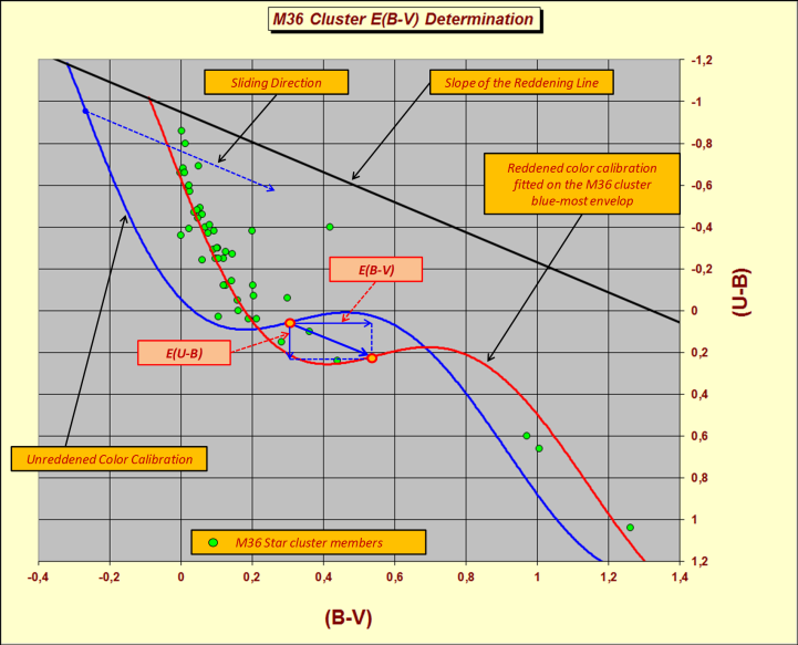
Fig. 1 – Sliding Fit Technique.
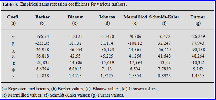
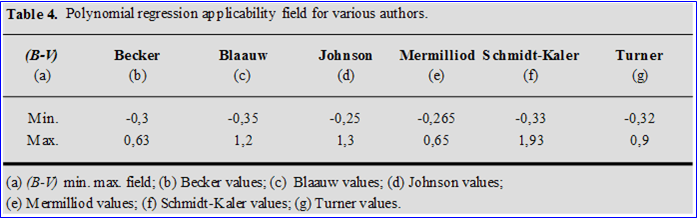
The general analytics shape for each empirical calibration on TCD is:
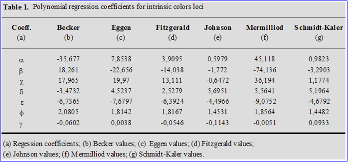
(U-B)o = a (B-V)o6 + b (B-V)o5 + c (B-V)o4 + d (B-V)o3 + e (B-V)o2 + f (B-V)o + g ( 1 )
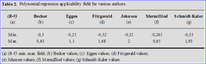
Where the equation (1) represents the intrinsic colors locus, while the values of the polynomial regression coefficients for several authors, are reported in table 1. In table 2 are shown the applicability fields for the 6th orders calibrations. Nevertheless, the Fitzgerald, Johnson and the Schmidt-Kaler empirical two color calibrations, cannot be well represented by a 6th order polynomial regression and a good fit with tabulated values occurs only when, at least, a 9th order polynomial is considered for regression. However the user must be advised that, the Excel polynomial regression lines are not Splines! For this reason and from a graphical point of view, the Runge's phenomenon is not avoided and certain oscillations can occur in the Excel graphical representation. In any cases, for every fits, the mathematical value is always the reference value!
II-b Individual reddening corrections procedures, intrinsic colours and individuals reddening lines.
The effect of the interstellar reddening causes a star to move, on TCD, to the right and down nearly parallel to the reddening line (RL). Now, it can be assumed that the distance between an observed point, on TCD, and the two color intrinsic calibration, calculated along its appropriate reddening line, yields the individual color excess E(B-V). At this purpose we define the RL as the locus where we find, sometimes scattered, stars of the same spectral class with the same intrinsic colors, but subjected to various degrees of interstellar absorption. The fundamental property of the RL consists in crossing the two colors calibration in a point that yields individual intrinsic colors, for the stars lying on it. Now, since in the UBV system the RL slope is known becomes possible to get the intrinsic colors of an observed star. From a rigorous point of view, the RL is not just a straight line and can be well represented by the following second order expressions:
E(U-B) = XE(B-V) + YE(B-V)2 ( 2 )
and the ratio between color excesses as:
E(U-B) / E(B-V) = X + YE(B-V) ( 3 )
In previous equations, X is the RL slope and Y its curvature.
The values commonly accepted for X and Y are: X = 0.72 and Y = 0.05 for OB
stars. Currently, however, the curvature factor of 0.05 seems quite inappropriate
for most star clusters and a 0.02 value for the curvature is considered more
corrected see Turner D. G. (1989, 1994). Therefore, while the curvature factor
Y appears to be constant along galactic plane, the slope varies from region
to region in the sky, assuming a medium value closer to X = 0.75. From an
operative point of view, to investigate the ratio E(U-B)/E(B-V) directly using
the available data, rather then assume the normal value, is a very important
point. The ratio can be evaluated providing very accurate spectral types and
luminosity classes, for a sample of cluster members. Thinking for a moment
over RL fundamental property, we can conclude that the process to find intrinsic
colors can be substantially reduced into a geometric matter. However, since
the analytics expression of the two color calibration is not surely linear,
but it can be well described by a 6th order polynomial, it’s clear that the
solution of the system can involve some difficulties. Therefore we can overcome
these difficulties, taking in consideration that the larger quantities of
stars within a young galactic open cluster are Early Type stars. So, as we
know from MK classification Morgan (1963), the population Early Type stars
belongs to the spectral classes O, B and early A types. Considering now, for
the reasons just said, only the intrinsic colors for early type stars, the
previous equation (1) can be reduced from a 6th order polynomial to a regression
line between the spectral classes O, B and early A. The Hr Trace code uses,
for default, the Schmidt-Kaler 1982 calibration on TCD and for this calibration,
we can express the feature concerning spectral classes O,B and early A with
the following regression line:
(U-B)o = 3.7082(B-V)o + 0.04 ( 4 )
So, the calculations of intrinsic colors for programmed Early Type stars in our open cluster, will consist in constructing a series of reddening lines with E(U-B)/E(B-V) slope eq. (3) that, connecting the observed positions with the intrinsic colors line equation (4), allow us to read the coordinates of intersection points. We just have to avoid RL application on TCD, where ambiguous solutions can be introduced by multiple intersections with the two color calibration. In any case and more generally, we can get an accurate determination of the intrinsic colors, if the TCD satisfies the requirement, according which, the slope of the RL must be as different as possible from the slope of the color calibration, in order to have the maximum separation between stars intrinsically similar, but affected by different degrees of reddening. Observing the TCD calibration, it’s easy to see that the previous condition is really true for stars from O5V to B9V, A3V to F4V and G6V to K0V spectral classes. Unfortunately the same requirement is not satisfied, on TCD, for stars from B9.5V to A2V and F5V to G5V spectral classes. It’s essentially for this last reasons that, in de-reddening Cepheids or yellow stars, the BVIc system must be preferred. At this purpose Dean, Warren and Cousins (1978) have derived the reddening free locus for Cepheids in the (V-I)c vs. (B-V) plane, calibrating the zero point from photoelectric observation of star inside cluster or associations, with well-known reddening values. They have found that the reddening slope and reddening index, in the (V-I) vs. (B-V), can be well represented with the following relations:
E(V-I)/E(B-V) = X[1+ 0.06(B-V)o +0.014E(B-V)] ( 5 )
and still
E(B-V) = Eo[1-0.08(B-V)o] ( 6 )
Here, X is given by the ratio E(V-I)/E(B-V) for one star with E(B-V) ? 0, while Eo is the color excess which a star with (B-V) = 0 would suffer, when observed through the same quantity of absorbing material.
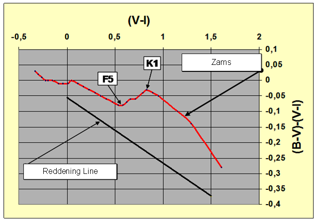
Figura 2 The (V-I) vs. (B-V)-(V-I) plane.
Plotting the color calibration and the appropriate reddening line in the (V-I) vs. (B-V)-(V-I) diagram we see that, this last one, is inclined with a good slope respect to color calibration itself, just in the spectral area F5 ÷ K1, that contains yellow stars see figure (2). Data for the red color calibration in figure (2) are derived from R.W. Walker (1985).The same question, that is how to find a late type reddening relative to that of an early type, but using only UBV system, can be evaluated taking in account that X = E(U-B)/E(B-V) for medium and late type stars is significantly different, from that of an early OB type stars. So, we can evaluate reddening for these stars following Schmidt-Kaler (1961) or Fernie (1963) with equation (7):
h = EB-V (Spectral Type) / EB-V (B0) = 0.97-0.09(B-V)o ( 7 )
II-c Computation of R = [Av / E(B-V)]
The total absorption in the visual magnitude V, can be obtained on the base of the following quantity:
R = AV / (AB – AV) ( 8 )
Were AV and AB are the absorption in V and B bands respectively. The observed quantities in term of magnitudes, are related to intrinsic quantities as:
BObserved = BIntrinsic + AB
VObserved = VIntrinsic+ AV
Now because E(B-V) = AB - AV, substituting in eq. (8) we have:
R = AV / E(B-V) ( 9 )
If we know spectral types for a good number of stars in a cluster, the ratio R of total to selective visual absorption can be evaluated Turner (1976). Practically, one uses the Johnson (1965) cluster method, under assumption that all stars within a cluster are at the same distance from us (Neglecting the depth of the cluster itself that can be considered tiny compared with its distance). Under this condition the distance modulus (V-Mv), where V is the observed visual magnitude, should be a constant except for the effects due to variable intra-cluster absorption, that is, within cluster volume itself. The value of R can be evaluated plotting (V-Mv) versus E(B-V), because the slope of the straight line which best-fits observational data gives the R value. A good value of R is important, because the ratio of the total to selective visual absorption enters directly in the calculation of the true distance modulus as shown by the following:
VO – MV = V – RE(B-V) – MV ( 10 )
In equation (10), VO is the visual magnitude without effects of interstellar absorption and MV is the absolute magnitude.
III - Some consideration on the automatic capture algorithm for the early type stars and possible errors during the individual dereddening procedure.
When a set of photometric UBV data is loaded by the user the code, during the graphical search of the <E(B-V)> parameter on TCD performs, in background, the analysis and the automatic capture of the Early Type stars found in the photometric sequences. At the same time the code calculates, always in background and using reddening line method, the individual values for the captured Early Type stars. To improve the understanding of this process some clarifications could be useful. Observing the Schmidt-Kaler intrinsic color tabulation, it’s easy to see the (B-V)o and (U-B)o variations through the luminosity classes V, III, II, Ib, Iab, Ia. From a quantitatively point of view, the intrinsic colors values for the luminosity classes V and III differs very little. So, replacing a normal giant with a main sequence star, during the automatic procedure for the determination of the intrinsic colors, will correspond to carry out a small and practically much negligible error, for O and B Early Type stars. The same confusion between a giant or main sequence star and a bright-giant of luminosity class II, can involve an error ranging between 0.01 to 0.04 magnitudes. Even bigger will be the error if a normal giant or main sequence star is confused with a super-giant belonging to Ib, Iab, Ia luminosity classes. Such an may vary in a range between 0.06 and 0.07 magnitudes for O and B Early Type. It's useless to say that errors of this entity can lead to determine wrong intrinsic colors, compared with those really observed.
III-a Perturbing phenomena on TCD.
The perturbing phenomena on the TCD are perceived by
the observer as an evident scatter of the photometric data along the various
reddening lines, especially along the RL concerning OB stars.
In 1975 Wallenquist, using a stars count technique, studied the presence of
dark matter inside the clusters and in the surrounding regions. As result
of his investigation he found variation in stellar densities practically on
all the considered clusters. On the base of the Wallenquist observations seems
therefore reasonable to argue that the observed stars deficiency can be mainly
due to presence of absorbing matter between cluster stars. It’s the presence
of this accidentally distributed matter inside clusters that cause the non-uniform
extinction phenomenon. Although the differential extinction can be considered
the main element that acts on the dispersion of photometric sequences, this
is not the only one and others processes can influence dispersion such as:
stellar evolution, stellar duplicity, stellar rotation, differences in chemical
compositions, dispersion in ages, dispersion in distances, presence of non
members and not last, the limited precision in de-reddened data Burki (1973,1975).
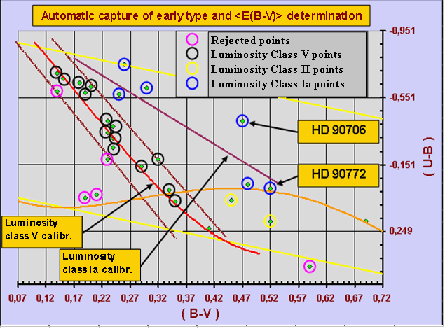
Fig. 3 - IC 2581 Mapping of automatic early type capture by dereddening algorithm
III-b Cases of low differential extinction.
The figure 3 shows the TCD for the southern cluster IC 2581 obtained plotting the original photometry of Lloyd Evans (1969). Over this chart are also shown:
· The best-fit between the two color Schmidt-Kaler intrinsic OB calibration
and IC 2581 OB sequence.
· The luminosity classes V stars within the black circles.
· The luminosity classed II and Ia stars respectively inside yellow
and blue circles.
Naturally, the distinction between the luminosity classes is not always therefore
simple as in the previous Figure 3, this because in the case of IC 2581, we
are not in presence of larger amount of differential extinction.
As we know from spectroscopic survey HD 90772 is an A7 Ia-O Super giant, using
the Schmidt-Kaler 1982 tabulation we can derive the HD 90772 intrinsic color
as follows:
(B-V)o = 0.12 and (U-B)o = 0.09 ( 11 )
Now, if we draw the HD 90772 individual RL using a normal slope value E(U-B)/E(B-V) connecting the position of this star on TCD, with the luminosity class V feature rather than with the equation that represents the (O,B,A) Ia intrinsic colors locus, we will find a wrongly B6V ÷ B7V star, rather than the more corrected A7Ia-O. This because in the first case, (intersection of the RL with the luminosity Class V intrinsic sequence), we will find the following intersection point:
(B-V)o = - 0.135 and (U-B)o = - 0.49 ( 12 )
While in the second case, (intersection of the RL with the luminosity class Ia intrinsic sequence), we will find:
(B-V)o = 0.13 e (U-B)o = 0.07 ( 13 )
It's necessary at this point to specify that Hr Trace, during the calculation of the intersection points as well as the luminosity classes uses a series of linear approximations as follows:
Luminosity class Ia: (U-B)o = 1.9543(B-V)o - 0.5839
Luminosity class Iab: (U-B)o = 2.3336(B-V)o - 0.4784
Luminosity class Ib: (U-B)o = 2.4553(B-V)o - 0.429
Luminosity class II: (U-B)o = 3.7742(B-V)o + 0.0177
This in order to determine the E(B-V) values and afterwards derives the intrinsic colors as:
(B-V)o = (B-V) - E(B-V). ( 14 )
Subsequently using the (B-V)o value, just determined,
inside a 6th order polynomial approximation to the intrinsic colors, the (U-B)o
for the considered luminosity class, is obtained.
It appears clearly that the de-reddening algorithm, beyond calculating the
individual E(B-V) values must also guarantee, when differential extinction
allows it, the correct interpretation of luminosity classes on TCD diagram.
A misinterpretation of the luminosity classes could not help us to isolate
with certainty, the main sequence stars class V, that the code must capture
and use to determine, not only the medium E(B-V) value, but also the medium
distance modulus for this stars group. On the other hand observing the previous
fig .(3), turns out obvious like HD 90772 belongs around the Ia luminosity
class.
III-c Cases of high differential extinction.
The methodology as soon as shown cannot be always used.
This is true particularly in presence of high differential extinction ( clusters
many young ). In this cases, the user can proceed determining first, differential
extinction value ?E(B-V) and after the cluster <E(B-V)> from this last
value. The effects of differential extinction are important in young cluster.
In fact, due to their young age, the interstellar nursery matter can be still
present inside the cluster itself.
A detailed discussion about the differential extinction in open clusters,
its effects and the treatment, can be found in Burki (1975). In any case,
in presence of similar scenarios, our code during E(B-V) calculation, will
consider that, for all Early Type those Johnson Q method value is less than
– 0.38 will exist a unique solution – intersection - between reddening line
RL and two color intrinsic calibration so, following Golay (1974) will be:
E(B-V) = (B-V) – [(U-B) – X(B-V) – 0.05(B-V)2 / 3.012-0.05(B-V)]. ( 15 )
III-d Particularly reddened sky fields.
In presence of heavily obscured regions or when particularly data dispersion on TCD gives impossible to obtain a correct value for cluster <E(B-V)> through the sliding fit technique, the user can always get the spectroscopic data using the Webda database connection link or the ADS literature query. With this data, turn out possible select and use the code spectroscopic de-reddening interface. These utility collecting associations between spectroscopy and photometric indexes allow us to obtain the variable extinction diagram. As already side, the ratio of total to selective absorption can be evaluated if we know spectral types of a good number of stars in the cluster. At this purpose the code spectral de-reddening interface uses the cluster method procedure as given in Johnson (1965). So, knowing spectral type and from this last ones the absolute magnitudes, we can derive the intrinsic colors and the color excesses. Further, one plots of (V-Mv ) versus E(B-V) gives us one observational distribution whose slope value is R. Note that the above procedure is useful only for stars that have already reached the main sequence.
IV - Determining the true distance modulus <Vo-MV>.
Star clusters are small enough compared with their distance. Thus we can assume that the cluster members are at the same distance from us. If this is a reasonable idea, the apparent magnitude of the cluster members V differs from their absolute magnitudes MV by the same amount V - MV and we can refer this quantity as the distance modulus. Plotting now the apparent magnitudes of cluster stars with respect to their spectral types or color indexes, the resulting array of points has the same significance of a spectrum or color index vs. absolute magnitude calibration, except for distance modulus difference. In determining the distance of a galactic cluster for photometric way, the method followed by Hr Trace, is the Zams fitting one. To hit this mark, the code uses various existing empirical calibrations such as: Becker & Fenkart (1971), Blaauw (1963), Eggen (1965), Johnson (1963), Mermilliod (1981), Schmidt-Kaler (1982), Turner (1981). All this empirical calibrations put in relation the de-reddened (B-V)o color index, with the absolute magnitude. Now, the distance modulus of any cluster can be obtained matching the comparable parts between our calibration and the cluster array in study on a (B-V)o, Vo diagram finding the difference between the apparent and the absolute magnitudes. This last operation can be obtained automatically or graphically making a sliding towards the bottom of our calibration until we have met the cluster array. In determining the distance modulus the code uses, for default, the Schmidt-Kaler 1982 empirical zams, that allows us to obtain the mathematical best-fit. As for the TCD interface, the Zams lines have been constructed with 6th orders polynomial interpolations of tabular values supplied by several authors. The zero age main sequence locus, according to general polynomial expression, can be well represented by equation (16) as follow:
Mv = a (B-V)o6 + b (B-V)o5 + c (B-V)o4 + d (B-V)o3 + e (B-V)o2 + f (B-V)o + g ( 16 )
While in tables 3 and 4 are shown, respectively, the regression coefficients and the applicability fields for the various authors. With the mathematical best-fitting procedure the code calculates, for all the captured Early Type photometric members in the TCD interface, the individual distance modulus (Vo-MV) and subsequently averaging over all (Vo-MV), obtains the medium true distance modulus <Vo-MV> for the cluster. The mathematical best-fitting wizard works only with the Schmidt-Kaler 1982 calibration, while for all other empirical calibrations (B-V)o, MV arranged by code, it's always possible to obtain a graphical fitting.
In the cases of graphical match, the user will proceed searching the best-fit to the cluster array with an eye to the scatter of the observed points and try to fit the less luminous envelop, from an evolutionary point of view, for members found on the Zams. If we superimpose, on a color – absolute magnitude diagram, several cluster as shown in Figure 4, we see that, practically, all arrays seems to born from an unique envelop line, under which there are only white dwarf. This line is referred as the Zams (Zero age main sequence) and the various array separation points have been called Turn-off points. Note also that from an evolutionary point of view, the zams envelop can be defined as the low luminosity locus Balona (1984).
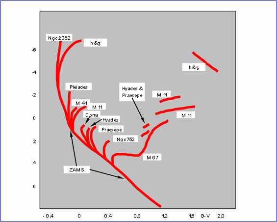
Fig. 4 - Composite Color-Magnitude diagram for various clusters
IV-a The IC 2581 <Vo-MV> determination.
Now we see, practically, how all we have previous said, can be obtained using the Hr Trace software. Observing the (B-V)o, Vo plane in Figure5, we see that the IC 2581 main sequence is very well defined in the interval from (B-V)o = -0.21 to (B-V)o = 0.17, while the blue Turn-off point is found around (B-V)o = -0.27.
The scatter in the observed points for IC 2581 is very low and this leaves us to preview a low (p.e.) as a result of the best-fit calculations (better adaptation to the points between empirical calibration and the IC2581 array). The value selected for the Turn-off point, will be used by the code to calculate the cluster age using: A. Maeder, G. Meynet, C. Mermilliod (1993) calibration. The figure 5 shows the starting situation, while the figure 6 shows the fit and the so obtained true distance modulus a value that turns out to be 12.35 ± 0.15 magnitudes. Following W. Becker (1963, 1966), we must repeat the same procedure in the Vo, (U-B)o plane and then average the values.
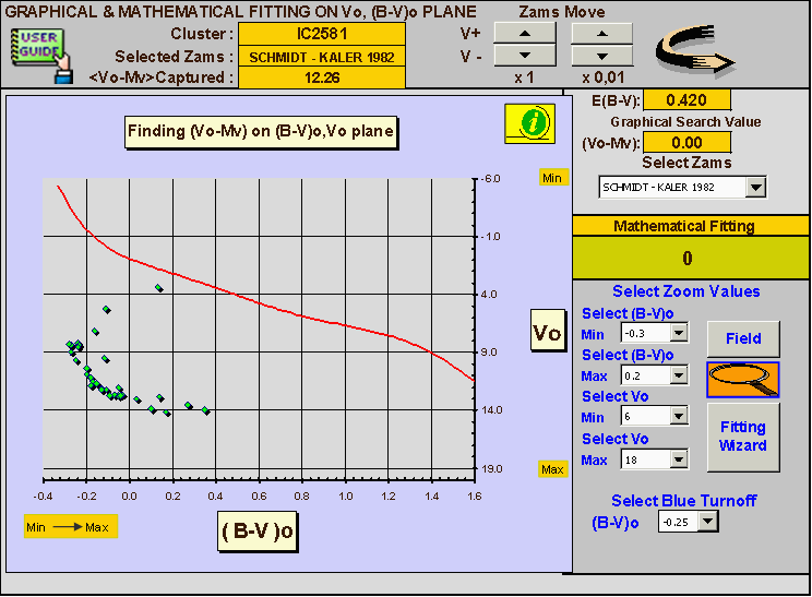
Fig. 5 Starting situation for distance modulus serach of IC 2582
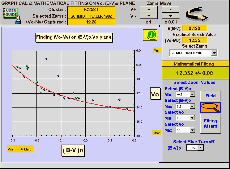
Fig. 6 Best fitting obtained from (B-V)o = -0.30 to (B-V)o = -0.20
IV-b Selection of cluster members question.
The determination of cluster membership is difficult and can be accomplished through various criteria. These criteria are: photometric, kinematics, statistical and spectroscopic. Nevertheless, as often it happens, inadequacy of statistical method or lacks of spectroscopic data limit strongly some of these methods. Moreover lack of spectroscopic data limit also the recognition of unusual cluster members and therefore, of astrophysical important objects. In any cases, the code does not account for membership analysis. This complex and not easy analysis is left to a preliminary study, which should eliminate spurious data before the running of the photometric analysis. Presence of spurious data increases the scatter and worsens the results! Nevertheless, on the clean data, the code performs the criterion for group membership as suggested by Walker (1965). This criterion states that a member should have a distance modulus no more than 0.5 mag. from the average modulus and the duplicity will not brighten a star more than 0.75 m. However, the Walker’s criteria it’s reliable only for main sequence stars.
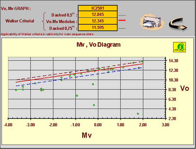
Fig.7 Application of Walker's criteria to IC 2581
IV-c The color magnitude diagram.
After the determination of the distance modulus, the code can calculate the absolute magnitudes and plot the color-absolute magnitudes (B-V)o, MV diagram fig. 7. The simple observation of this figure, shows that IC 2581 is a young galactic cluster formed by young stars, with superficial temperatures ranging between 8000° K to 40000° K. Even the photometric radii are considerable, the values calculate by Hr Trace using Wesselink (1969) calibration fall in the range between R/RS = 2.2 to R/RS = 280. The maximum values calculate by Hr Trace are those of HD 90772 and HD 90706, two super giants showing high absolute magnitude Mv = -8.96 and Mv = -7.16 respectively, but with similar bolometric magnitude Mbol = -8.93 and -8.60. In a recent study of this cluster D. Turner found for the two mentioned stars the following values: : Mv= -8.8 and Mv = -7.2 respectively based on a distance modulus equal to 12.29 ± 0.10. Our results are also in good agreement as a comparison between spectral and photometric classifications.
It's also interesting to observe the relationship between the photometric radii of these two stars, that turn out to be (HD 90772 / HD 90706) = 3.67. The relationship between the radii of two super giants, must be considered according to the effective temperature of two stars, that is calculated by Hr Trace in 8033°K for HD 90772 and 14327°K for HD 90706. Evidently the colder body HD 90772, needs a huge radiating surface of warmer body HD 90706, in order to reach the absolute magnitude of Mv = - 8.96. This situation is very well explained by the Stefan-Boltzmann law (17):
L = 4pR2 sT4 ( 17 )
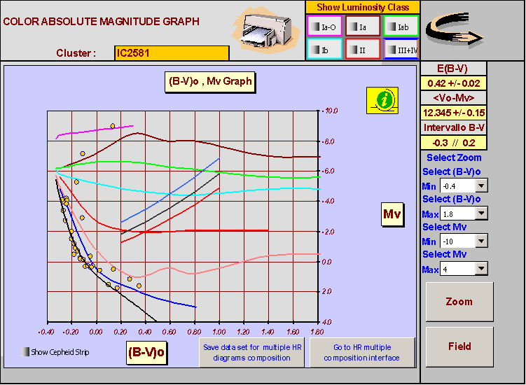
Figura 8 IC 2581 color-absolute magnitude diagram.
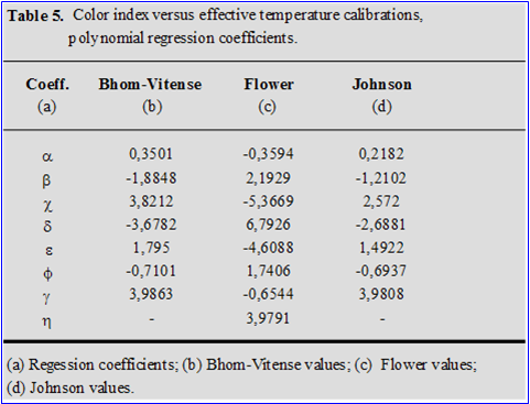
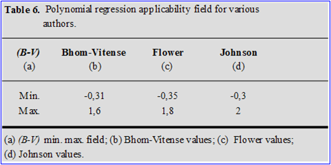
V - The HR theoretical diagram log (L/LS), log (Teff) and log (Teff ), MBol.
For the theoretical plane the code uses, in order to convert the observed intrinsic colors, various effective temperature tabulations such as: Bohm-Vitense (1981), H.L. Johnson (1965) and P. Flower (1975, 1977, 1996). The polynomial equation used to obtain the Teff values from the intrinsic color index is similar to the previous ones:
Log Teff = a (B-V)o6 + b (B-V)o5 + c (B-V)o4 + d (B-V)o3 + e (B-V)o2 + f (B-V)o + g ( 18 )
In particular for the P. Flower calibration, a 7th degree term was necessary:
Log Teff = a (B-V)o7 + b (B-V)o6 + c (B-V)o5 + d (B-V)o4 + e (B-V)o3 + f (B-V)o2 + g (B-V)o + h ( 19 )
The calculation of the amount Log (L/LS) is, on the contrary, is obtained through equation (20):
Log (L / LS) = 4.72 – [( Vo + BC – DM ) / 2.5] ( 20 )
Where BC is the bolometric correction and DM is the true distance modulus <Vo-MV>. The transition from the color-magnitudes CM diagram to the HR diagram requires transformation of the color index onto the effective temperature and absolute magnitude onto the bolometric magnitude. In both cases the rheology followed by the code to make calculations, is always the same. In the next tables 5 and 6 are shown the transformations coefficients.
The relation between the absolute magnitudes to the bolometric magnitudes is the following:
MBOL = Mv + BC ( 21 )
The bolometric correction is determined by Hr Trace using the H.L. Johnson (1966) and the P. Flower (1996) LogTeff., BC tabulations. Once obtained the conversions, the data are available through an appropriate theoretical interface in order to compare our calculations with a series of stellar models as can be seen in figs. 9 and 10.
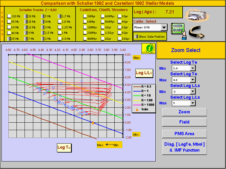
Fig. 9 - IC 2581 theoretical HRD Log (Teff), Log(L/Ls)
The superimposition of the evolutionary tracks from stellar models on the IC 2581 array, clearly shows that the majority of the members of this cluster are formed by stars found in the range between 2 to 15 M¤. Only HD 90772 and HD 90706 have been found in the range between 30 to 40 M¤, as we could expect considering the highest absolute magnitude of these stars. The yellow-red triangle on the diagram shows, for comparison, the solar position. In the same interface the cluster age from the blue turn-off value, using the A. Maeder-G. Meynet and C. Mermilliod (1993) calibration, is also obtained.
Afterwards without exit from this interface we can superimpose, on the cluster sequence and for preliminary evaluations, all a series of isochrones from V.Castellani, A.Cheffi and O.Straniero (1993) stellar models in the range between 30 Myr to 10 Gyr. More advanced analysis are possible using Teff, Mbol diagram of fig. 10, where we observe HD 90772 and HD 90706 to reach a bolometric magnitude Mbol = -8.96 and -8.60 respectively.
Moreover, on Log (Teff), Mbol interface it's possible to compare our clusters with the tracks from the stellar models of Geneva group Schaller & other (1992) for metallicity Z = 0.02 and Z = 0.001 and Padova group Bertelli & other isochrones (1994), for metallicity Z = 0.02, Z = 0.008 and Z = 0.004. Always from this interface, the user can start calculations with the aim of obtain value for the cluster PDMF ( Present Day Mass Function). The actual software release don’t allow for IMF ( Initial Mass Function ), but one patch focused in solving this problem is now under development.
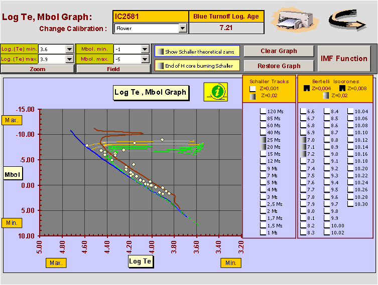
Fig. 10 - HRD Log (Teff), Mbol for IC 2581
V-a Variability phenomena inside Open Clusters.
Stellar variability studies inside or around open clusters, could disclose interesting possibilities for serious amateurs. This because, inside clusters, we can find various types of variable phenomena concerning population I stars. The user can identify variable objects using both LogTeff, Mbol and Massive Regions & Instability Strips interfaces. It’s possible, for instance, take in consideration variable objects lying over, or immediately around the main sequence, like ? cephei, as well as, SPB (Slowly pulsating B stars), or ? scuti. On the other hand, within very young clusters, the user can meet variability related to very massive objects such as: LBV, S Doradus, Wolf-Rayet, OB massive stars; while inside intermediate age clusters we can find variability connected to yellow super-giants or population I cepheids. Sometime young and intermediate age clusters can also contain some evolved objects like red super-giants with all their variability phenomena. Finally in clusters many young, there is also the possibility to study T-Tauri stars, another class of eruptive variable related to pre-main sequence phase or newly formed stars. T-Tauri variability is mostly due to flares phenomena. Also the study of binary stars in clusters can produce other important results. Concerning binary stars we know that, arranging together spectroscopic and photometric data, turn out to be known also the distance. Beyond this, some categories of variable stars, if members of the clusters, allow us to compare, whenever possible, the resulting zams fitting distance. We can compare distances, for instance, using the Period-Luminosity relations. A good example of those comparisons for contact binaries can be seen in Mochejska B.J. & Kaluzny J. (1999). In their work on the intermediate age open cluster Ngc 7789, they found some W Ursae Majoris systems in the cluster field. To asses cluster membership for contact binaries, the authors have applied the Rucinski & Duerbeck (1997) absolute magnitude calibration as follow:
Mv = -4.44 Log P + 3.02(B-V)o +0.12 ( 22 )
Where P is the contact binary period in days.
As results of calculation using equation (22), they discovered over 35 contact binary in Ngc 7789 cluster field. Of this 35 system, at least five seems to be cluster members with computed distance moduli within ± 0.2 of the cluster modulus. Naturally, similar comparisons can be done considering, for instance, d scuti and classical Cepheids whenever possible.
VI – a Some Examples – Cepheid’s & instability strip.
The NGC 129 Cepheid’s member it is caught while crossing the instability strip blue loop. See figure 11 that shows the crossing in the MBol , LogTe diagram (Green tracks Bertelli isochrones). DL Cass is also detected inside Cepheid’s instability strip in the interface Massive regions & Instability Strips. See Figure 12.
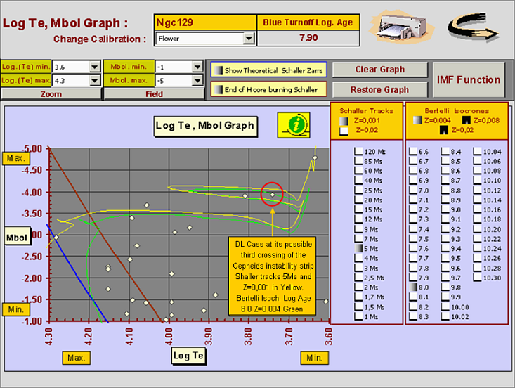
Fig. 11 Ngc 129 cepheid member DL Cass. On theoretical HRD
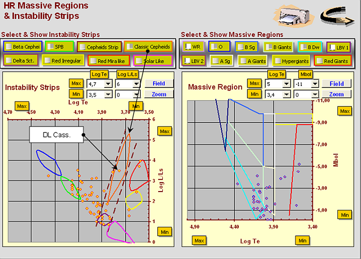
Fig. 12 - Hr Massive Regions & Intability Strips.
VII - a Some Examples – Comparisons between various clusters.
Comparisons between various clusters are available through a devoted interface for this type of analysis, see previous figure 13 where the twin clusters IC 2581 and NGC 457 are shown in comparison.
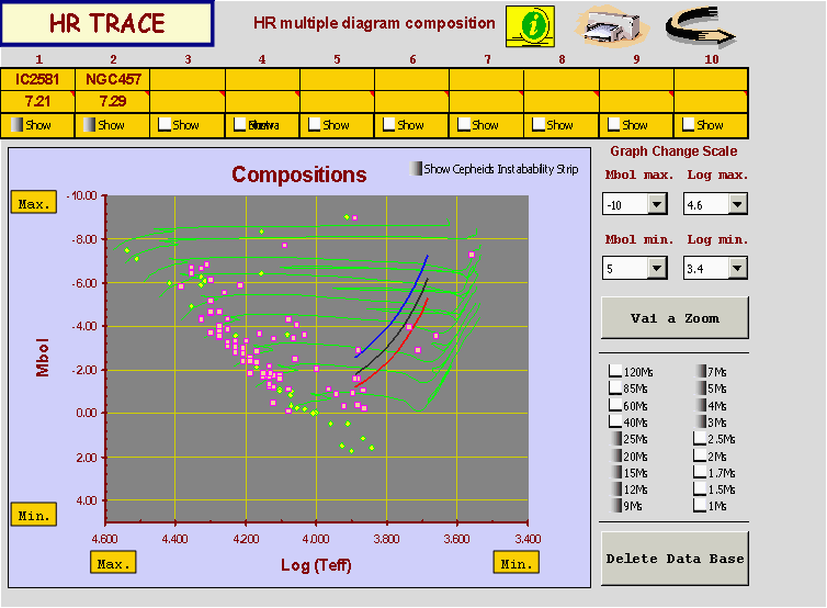
Fig. 13 – Hr multiple composition diagram.
Many other performances are available for the analysis of intermediate and advanced age clusters. There are some cases of targets observed through particularly reddened sky fields, where it's impossible to get individual E(B-V) value with the photometric way alone like in the case of the default cluster Stock 2.
VIII - a Interesting possibilities with intermediate and advanced open clusters.
Last
but not least, an interesting possibility still feasible for amateur instruments
is the research, within intermediate and old open cluster, of stars with medium
or even high degree of metallicity. This is quite simple, because these stars
appear well confined above the standard two color calibration, in the range
0.3≤(B-V)≤0.6 on TCD diagram.
In
a recent study Fischer & Valenti (2005) have obtained a relation between
the metallicity of the central stars and the probability that the environment
around this stars host planets. The relation is the following:
PPLANET =
0.03[(NFe/NH)STAR / (NFe/NH)SOLAR]2
This
means that stars with high metallicities are more likely to host planets.
Thus this search could be absolutely possible and aimed to specific target
instead of randomly searching. At this purpose, there are a lot of open clusters
with metallicities between -0.1 ≤FeH ≤-0.45, both in northern
and southern hemisphere to look for planetary search that are suitable for
new discoveries.
![]()
![]()
![]()
References & Bibliography.
Balona L.A. & Altri 1984 “ A re-calibration of the luminosities of Early Type stars: its effect on the Cepheid luminosity scale “ Month. Not. of the Roy. Astr. Soc. Vol. 211, p.375
Becker W. 1963 “ Die raumliche verteilung von156 galaktischen sterhaufen “ Zeit. fur Astrophys. Vol. 57, p.117
Becker W. 1966 “ Bemerkungen uber das verhaltnis der intersetellaren absorption “ Zeit. fur Astrophys. Vol. 64, p.77
Bertelli G. & other 1994 “ Theoretical isochrones from models with new radiative opacities “ Astron. & Astrophys. Supp. Vol. 106, p.275
Blaauw A. “ The calibration of luminosity criteria “ Basic Astronomical Data Ed. K. AA. Strand 1963, Chicago U.P.
Blaauw A. 1973 IAUS 54 " Problems in Calibration of Absolute Magnitudes and Temperature of Stars " Ed. Hauck & Westerlund ."
Bohm-Vitense E. 1981 " The effective temperature scale “ Ann. Rev. Astron. & Astrophys. Vol. 19, p.295
Burki G. Maeder A. 1973 " On the use of UBV photometric diagrams for inferring the existence of an open star cluster “ Astron. & Astrophys. Vol. 25, p.71
Burki G. 1975 " Non uniform extinction in open star clusters and dispersion of the photometric sequences “ Astron. & Astrophys. Vol. 43, p.37
Castellani V. Chieffi A. Straniero O. 1993 “ Evolution through H and He burning of galactic cluster stars ” Astrophys. Jour. Supp. Vol.78, p.517
Dean J.F. Warren P.R. & Cousins A.W.J. 1978 “ Reddening of Cepheids using BVI photometry “Mont. Not. Roy. Astr. Soc. Vol. 183, p.569
Eggen O. J. 1965 “ Some observational aspects of stellar evolution “ Ann. Rev. Astron. & Astrophys. Vol. 3, p.235
Fernie J.D. 1963 “ Intrinsic colors of supergiants “ Astron. Jour. Vol. 68, p.780
Fitzgerald P.M. 1970 “ The intrinsic color of stars and Two-Color reddening lines “ Astron. & Astrophys. Vol. 4, p.234
Flower P. J. 1975 “ Bolometric corrections for late type giants and supergiants “ Astron. & Astrophys. Vol. 41, p.391
Flower P. J. 1977 “ Transformation from theoretical HR diagrams to CM diagrams “ Astron. & Astrophys. Vol. 54, p.31
Flower P. J. 1996 “Transformation from theoretical HR diagrams to CM diagrams: effective temperatures, B-V colors and bolometric corrections “ Astrophys. Jour. Vol. 469, p.355
Giaccaglini G. " Excel 2000 VBA " Jackson
Harris M. " Microsoft Excel 2000 programming in 21 days " Apogeo & Sams Publishing.
Heintze J. R. W. 1973 IAUS 54 " Problems in Calibration of Absolute Magnitudes and Temperature of Stars " Ed. Hauck & Westerlund .
Jaschek C. e Jaschek M. " The Classification of Stars " Cambridge U.P.
Johnson H.L. 1954 " Galactic clusters and stellar evolution “ Astrophys. Jour. Vol. 120, p.325
Johnson H.L. 1957 " Photometric distances of galactic clusters “ Astrophys. Jour. Vol. 126, p.121
Johnson H.L. & Morgan W.W. 1953 “ Fundamental stellar photometry “ Astrophys. Jour. Vol. 117, p.313
Johnson H.L. & Hiltner W.A. 1956 “ Observational confirmation of a theory of stellar evolution “ Astrophys. Jour. Vol. 123, p.267
Johnson H.L. “ Photometric system ” Basic Astronomical Data Ed. K. AA. Strand 1963, Chicago U.P.
Johnson H.L. 1965 “ Interstellar extinction in the galaxy “ Astrophys. Jour. Vol. 141, p.923
Johnson H.L. 1966 “ Astronomical measurements in the infrared “ Ann. Rev. Astron. & Astrophys. Vol. 4, p.193
Lloyd Evans T. 1969 “ The open cluster IC 2581 “ Mont. Not. of the Roy. Astron. Soc. Vol. 146, p.101
Mermilliod J. C. 1981 “ Comparative studies of young open clusters ( III ) – Empirical isochronous curves and zero age main sequence “ Astron. & Astrophys. Vol. 97, p.235
Meynet G. Mermilliod J.C. Maeder A. 1993 “ New dating of galactic open clusters “ Astron. & Astrophys. Supp. Vol. 98, p.477
Mochejska B.J. & Kaluzny J. 1999 “ Variable stars in the field of the open cluster Ngc 7789 “arXiv:astro-ph/9907272 v1 20 jul. 1999”
Moffat A.F.J. 1974 “ On the ratio of total to selective absorption in the open cluster IC 2581 “ Astron. & Astrophys. Vol. 32, 103
Morgan W.W. e Keenan P.C. 1973 “ Spectral classification “ Ann. Rev. Astron. & Astrophys. Vol. 11, p.29
Pesch P. 1959 “ The galactic cluster Ngc 457 “ Astrophys. Journ. Vol. 130, p.764
Rucinski S.M. & Duerbeck H.W. 1997 Publ. Astr. Soc. Pacific Vol. 109, p.1340
Schaller G. & other 1992 “ New grid of stellar models from 0.8 to 120 solar masses at Z = 0.020 and Z = 0.001 “ Astron. & Astrophys. Supp. Vol. 96, p.269
Schmidt-Kaler T.S. 1961 “ Die verfärbung als function der interstellaren absorption und der energieverteilung des kontinuierlichen sternspektrums ““ Astron. Nacth. Vol. 286, p.113
Schmidt-Kaler T.S. “Landolt-Bornstein” Group 6 Vol. 2b, 1982 Springer Verlag
Turner D.G. 1973 “ Differential reddening in the open cluster IC 2581 “ Astron. Jour. Vol. 78, p.597
Turner D.G. 1976 “ New determination of R in open clusters “ Astron. Jour. Vol. 81, p.1125
Turner D.G. 1978 “ The value of R in IC 2581 “ Astron. Jour. Vol. 83, p.1081
Turner D.G. 1979 “ A reddening free main sequence for the Pleiades cluster “ Pub. of the Astron. Soc. of Pacific Vol. 91, p.642
Turner D.G. 1981 “ Comments on the cluster main sequence fitting method. ( I ) The distance of Ruprecht 44 “ Astron. Jour. Vol. 86, p.222
Turner D.G. “ Comments on the cluster main sequence fitting method. ( II ). A re-examination of the data for Ngc 6649 and the Cepheid V367 Scuti “ Astron. Jour. Vol. 86, p.231, 1981
Turner D.G. 1989 “ Comments on the cluster main sequence fitting method. ( III ). Empirical UBV reddening lines for Early Type stars “ Astron. Jour. Vol. 98, p.2300
Turner D.G. 1994 “ Demonstrating cluster main sequence fitting to best advantage “ Jour. of the Roy. Astron. Soc. of Canada Vol. 88, p.176
Turner D.G. 1996 “ The progenitors of classical Cepheid variables “ Jour. of the Roy. Astron. Soc. of Canada Vol. 90, p.82
Turner D.G. 1996 “ Monitoring the evolution of Cepheid variables “ JAAVSO Vol. 26, p.101
Walker R.W. “ CCD photometry of galactic clusters containing Chepeid variables “ Mont. Not.of the Roy. Astron. Soc. Vol. 213, p.889
Wesselink A.J. 1969 “ Surface brightness in the UBV system with applications on Mv and dimension of stars “ Mont. Not. of the Roy. Astron. Soc. Vol. 144, p.297
![]()
![]()
![]()