![]()
Effects of Earth Atmosphere. Some Definitions
Transmission of the Earth atmosphere
The atmospheric transmission law can be defined as follows:
Tn µ e a
where a µ air column density along the line of sight.
Earth Airmass plane parallel approximation
The Airmass is defined as the ratio (k / ko) of air column density, to the value at the zenith ko. For a plane parallel atmosphere the airmass is expresed by the following equation: airmass = X(z) = sec(z), where z = zenith distance.
sec(z) = (cos f cos H cos d + sin f sin d) -1
with H = star's hour angle, d = star's declination and f = observer's latitude.
Earth Airmass curvature layers approximation
To account for Earth atmospheric curvature layers effects, is frequently used the following equation:
X(z) = secz - 0.0018167(secz-1) - 0.002975(secz-1) 2- 0.000808(secz-1) 3
Overview on data reduction - Absolute Photometry -
To get accurate results data reduction is necessary. This procedure can be outlined as follow:
Point ( 1 ) Correct for background and determination of instrumental magnitudes
Consist in a subtraction for each star in each of the tree filter U,B,V the appropriate background and subsequent proceed to calculation of instrumental magnitudes u, b, v, and colours (u-b), (b-v).
Point ( 2 ) Solve for extinction
First obtain the airmass X(z) for each star using previous illustrated formulas and than procced to determination of extiction coefficents through the following plots of extinction data: v vs. X, (b-v) vs. X, (u-b) vs. X whose slopes are respectively Kv, Kbv and Kub extinction coefficents.
Point ( 3 ) Correction of measurements
Correction of all measurements as follow:
Point ( 4 ) Coefficents determinations
Determinations of q,w,t and JV, JBV, JUB coefficents, using standard stars as follow:
Point ( 5 ) UBV Standardization Equations
Application of standardization equations to all programmed stars
Generality on Photometric Systems
Any photometric system is an instrumental system in the sense that it is completely defined by specifying the detector characteristics, the bandwitdh of filters used ( sensitivity functions ) and a series of standard calibration stars.
All photometric systems can be divided into three categories that are essentially based on the filters transmission and the window size of the wavelenght interval transmitted.
On this bases the three rough categories are:
Broad-band and intermediate-band filters
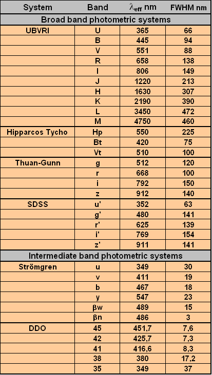
The UBV system and broadband filters
Between all possible systems, the UBV system has became immediately the most popular among astronomers. Since its first definition by H.L. Johnson and W.W. Morgan ( Ap.J 114, 522 and Ap.J. 117, 313 ). This system was thought to be closely tied to the MK system of spectral classification. In fact it was developed for the photometric study of the stars classified in the Yerkes system. Substantially It uses three wide passbands called U (ultraviolet), B (blue) and V (visual) each about a thousand angstroms wide. Central wavelenght of the three filters are approximatively those shown in tab 1:
| Band |
<
l > Å |
Dl
Å |
U |
3650 |
660 |
B |
4450 |
940 |
V |
5510 |
880 |
Tab 1 - Three UBV bands.
While sensitivity function S(l) for the three filters tab 2 are:
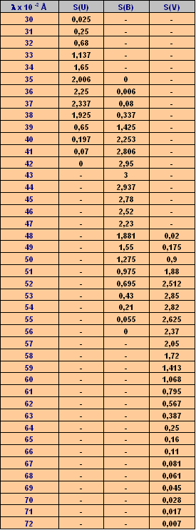
Tab 2 - UBV filters response functions.
I apologize for the use of the Italian notation in Tab. 2. The commas should always be read as dots.
The response function in tab 2 valid for one airmass, is taken from appendix ( A ) in Matthews & Sandage 1963 Ap.J. 138, 30. In that job authors focused their attention over the intersting problem of compute UBV colors of radiant sources with given energy distribution. This can be done when trasmission functions S( l ) of the U,B,V system are known. Application of this methodology allows us, for instance, to compare between observed and computed colors.
Particularities of the UBV system
From an instrumental point of view, the UBV system was deveoped in the fifties around the RCA 1P21 photomultiplier tube and three band filters. THis means that for any evaluations, we must consider the complessive interaction betwen the photomultiplier response and the response of the filters. To understand the complessive reology and try to obtain some conclusion, we plot first: the spectral response of the three filters on a normalized transmission scale figure 1 and than, the RCA 1P21 photomultiplier response function figure 2. Finnally the fig. 3 shows the superposition of entire intrumental UBV system filters plus the 1P21 response functions.
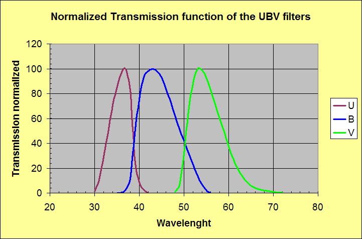
Figure 1 - UBV filters normalized transmissions functions.
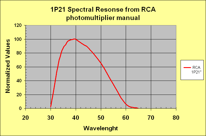
Figure 2 - RCA 1P21 normalized transmissions function.
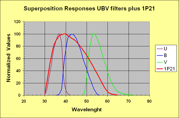
Figure 3 - RCA 1P21 and UBV filters normalized transmissions functions.
Looking to figure 3, we can see how this system is not complete determined by its filters or by combined action of the photomultiplier and the filters. The short wavelengt cutoff is, in fact, totally determined by earth's atmopheric ultraviolet window and on the opposite side, longh wavelenght cutoff, is found on the left side of the natural response curve of the photomultiplier 1P21. Naturally on the short wavelenght side, the atmospheric cutoff can create some difficulties in relation to the observatory's altitute.
Some Problem with U filter and (U-B) color index
Johnson U filter is centerd at 3600 A and it has a red leak that transmit some light in the near infrared. This transmision should be known so that it can be bloked or subtracted from measurement obtained through this filter. Besides in the continuum of stellar radiation at the wavelenght of 3646 A occurs the Balmer discontinuity those size is function of spectral type and luminosity class. In dealing with UBV system this discontinuity must be examined, because U passband extends partially across the discontinuity. So variation in discontinuty's strenght shift the effective wavelenght of this filter in the sense that the greater the discontinuity, the larger the effective shift ( Moffat & Vogt 1977 Pasp 89, 323 ). All this can create various difficulties for the exctinction coefficent used to reduce instrumental U magnitudes to the standard system. Another problem may be represented by a mismatch between UBV system filter used in comparison with the standard UBV passbands defined by Johnson, this because the original system and its standard stars was originally defined by Johnson's photometer. In other word the UBV system is the istrumental system of that photometer (1P21+Filters). Thus any observations with a different instrument and filter system, such as modern CCD camera, can produce the risk of mismatch with the standard original Johnson system. Further and more advance discussions on this arguments can be find by the reader in Bessel 1990, Pasp 102, 656-1181, while more rigorous analysis of problem of standardizing U band with CCDs can be find in Straizys & Lazauskaitè 1995 Baltic Astronomy 4, 88.
UBV standard stars and zero points
Originally the system was defined by 10 primary standard and zero points by the following six stars: a Lyr, a Crb, g Oph, g Uma, 109 Vir and HR 3314 whose average color index is defined to be zero as:
(B-V) = (U-B) = 0
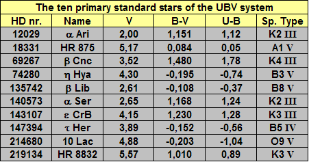
Tab. 3 - The 10 primary standard of the UBV system.
I apologize for the use of the Italian notation in Tab. 3. The commas should always be read as dots.
Standard stars are required to compare the different observers results with each other. This is because each instrumental system has its own observational response function, so that the same stars will not have the same brightness using different instrumental systems. The difference in response levels results from various factors ranging from:
To get around this series of problems, the existence of a standard stars system give possible to calibrate any new observations against the known brightness of the std. stars. Infortunately neither previous 10 primary, nor the stars in secondary list published by Johnson ( 1963 Basic Astronomical Data pag. 209 ) can be used with modern CCD cameras since they are very luminous ( very luminous target causes saturation of ccd images also with little exposition times ). Thus to calibrate and standardize our measurement with a system composed by UBV filters and a ccd camera we must refer to the following links, where we can find catalogues and lists of stadard stars.
Data bases links
Arizona edu Standard Stars Atlas Info
CDS - Galadi+ 2000 UBVRI-CCD Secondary Standard Stars near Landolt Fields -
SOFA - Standard Objects For Astronomy - Astro.Utoledo.edu
Some useful publications
Bruce L. Gary - Transformation Equations
R.F.Garrison The Brightest Stars
Calibrating Photometry from instrumental to standard magnitudes with Excel
Normally astronomers use for the transformation of intrumental magnitudes into standard system magnitudes, the appropriate IRAF tasks. IRAF uses standard UBV colors and magnitudes as well as air masses to generate the trasformation equations. Nevertless for our purpose can be more easy use an Excel file to compute the transformation instead of IRAF tasks, simply adopting a linear relation of the following type:
dM = Mins - Mstd = a (B-V)std + b ( 1 )
Where: Mins = instrumental magnitude and Mstd = standard magnitude, while (B-V)std = standard B-V color and a and b are constants. Now if we plot on a chart the relation between dM and (B-V)std for each frame, the values of a and b can be determined simply using the Excel linear fitting tool. At this point the next two steps will be solve the following equations for V and B color:
Vins - Vstd = a (B-V)std + b ( 2 )
where Vins = Vinstrumental magnitude and Vstandard = Vstandard magntude and still
Bins - Bstd = c (B-V)std + d ( 3 )
where always Bins = Binstrumental magnitude and Bstandard = Bstandard magntude, now subtracting eq. ( 3 ) from eq. ( 2 ) we have:
(B-V)ins - (B-V)std = ( c - a ) (B-V)std + d - b ( 4 )
and rearranging
(B-V)std = [ (B-V)ins + b - d / 1 + c - a ] ( 5 )
This last result eq. ( 5 ) permits, simply, the transformation of the instrumental B-V to the standard system.
Relation between photometry and spectroscopy
Spectral classification is one of the most important topic in stellar astronomy. Is essentially for this reason that Johnson & Morgan have tried to obtain a sort of spectral classification using UBV photometry. UBV system is, in fact, close tied to MK spectral classification and the B-V color index is related directly to MK spectral type and temperature, as we can see in the following two figures 4 and 5:
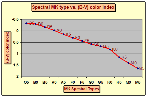
Fig.4 - Relation between (B-V) color index and MK spectral Types
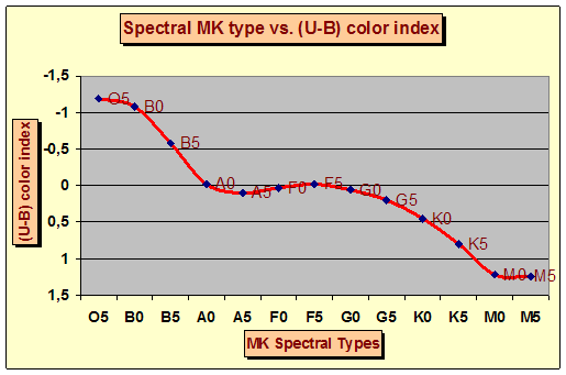
Fig.5 - Relation between (U-B) color index and MK spectral Types
In both previous figures we can see a very definite relation and almost very linear phat over the whole MK spectral range, aboveall between (B-V) color index and MK types. The (U-B) color index shows a similar linear shape only in the range B0 - A0 and due to its favourable slope in this spectral range, (U-B) color index seems very useful in discriminating early B type stars with respect (B-V) color index.
![]()
![]()
© 2006 - Valter Arnò.