Empirical Calibration Usage - An Example with A. Blaauw Zams -
![]()
![]()
Generality
Rerading the literature we find, practically always, all the empirical calibrations expressed in tabular form. So, to be able to use this calibrations in our calculations, we must transform tabular functions into analytical forms. Using both statistical methods and an Excel sheet, the procedure to obtain each empirical calibration analytical form can be outlined as follow:
So for a linear regression, the expected Excel fitting equation should be:
Y = aX + b
Where a and b are the linear regression coefficents.
While in the case of a polynomial regression - for instance a 6th order - the analytical shape should be:
Y = aX6 + bX5 + cX4 + dX3 + eX2 + fX + g
Where a, b, c, d, e, f, g are the polynomial regression coefficents.
Regression using an Ms Excel chart and Trend Analysis
An Excel trendline within a set of empirical data, shows just the trend of data. Taking in considearation the A. Blaauw Zams (B-V)o, Mv empirical calibration, an analytical relation by fitting data values derived from an empirical calibration can be obtained as follows:
The tabular form fot the Blaauw Zams (B-V)o, Mv is represented in the following table:
|
( B-V )o |
Mv |
-0,35 |
-5,50 |
-0,30 |
-3,30 |
| -0,25 |
-2,10 |
-0,20 |
-1,10 |
-0,15 |
-0,20 |
-0,10 |
0,60 |
-0,05 |
1,15 |
0,00 |
1,55 |
0,05 |
1,80 |
0,10 |
2,00 |
0,15 |
2,25 |
0,20 |
2,50 |
0,25 |
2,70 |
0,30 |
2,95 |
0,35 |
3,20 |
0,40 |
3,55 |
0,50 |
4,20 |
0,60 |
4,80 |
0,70 |
5,40 |
0,80 |
5,90 |
0,90 |
6,30 |
1,00 |
6,80 |
1,10 |
7,20 |
1,20 |
7,65 |
Table 1 - A. Blaauw empirical Zams (B-V)o, Mv
Now plotting on a XY type chart the previous A. Blaauw zams one can obtain the trend visible in fig. 1:
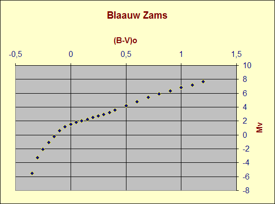
Fig. 1 - Excel first representation of A. Blaauw Zams
Now to obtain the usual representation of Blaauw Zams, click on chart Y axis and select values in reverse order see fig. 2
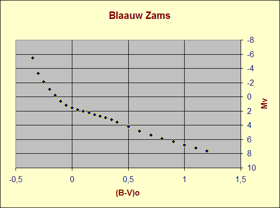
Fig. 2 - Usual A. Blaauw Zams representation
To add a trend line, right click on any data point of fig. 2 then select: "Add Trendline" within the showed popup, wait until the trendline dialog form is loaded and then select: "6th order polynomial regression type". Now using this funcyion option panel select: "Display Equation plus Display R-squared value on chart", then click ok button. The result can be seen in the following fig. 3
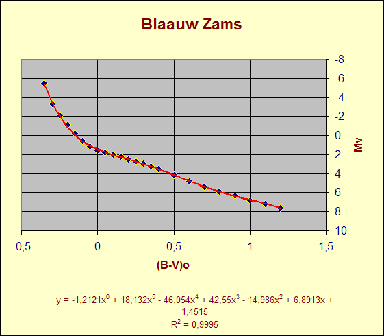
Fig. 3 - A. Blaauw Zams fitted by a 6th order polynomial trendline
With the previous procedure we have obtained an analytical expression. Analytica expression that relates data of table 1. This analitycal expression can be subsequently used in our calculation as follow:
Mv = -1,2121(B-V)o6 +18,132(B-V)o5 -46,054(B-V)o4 +42,55(B-V)o3 -14,986(B-V)o2 +6,8913 + 1,4515 ( 1 )
Being equation (1) the analytical form of the A. Blaauw empirical zams, a star showing an intrinsic color (B-V)o = -0,27 should shine with an absolute magnitute equal to: Mv = -2,6104.
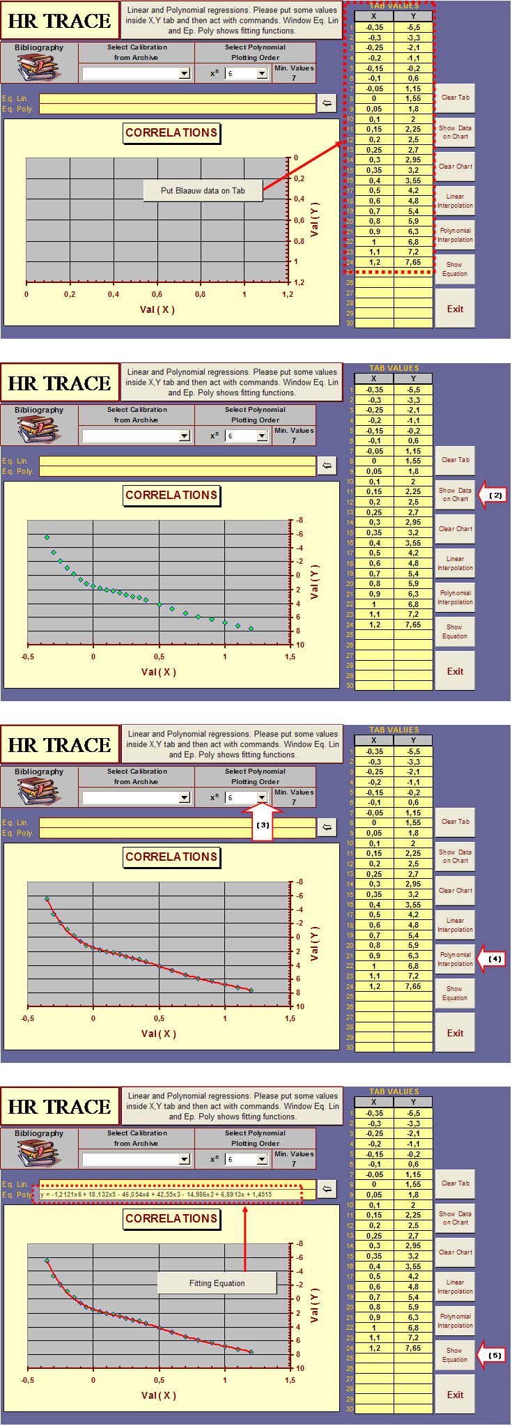
The same previous results can be easily obtained in 5 steps using the Hr Trace Lab Tool, downlodable through this site.
![]()
![]()
© 2006 - Valter Arnò.